Face Presence

Approach

How much of an infant’s recorded day contained a visible face?

• Unit: the video timeline. Face presence is a property of the infant’s view, not of any individual person, so two co-visible faces do not make the view twice as face-filled. Durations are therefore a wall-clock union: intervals are merged before summing.
• This differs deliberately from the FACS configuration analyses, which use person-time, because a configuration belongs to a face while presence does not.
• Denominator: total session duration (not valid_fullface). The question is what fraction of the recorded day had a face, so occluded and face-free time both belong in the base.

library(tidyverse)
library(brms)
library(easystats)
library(ggeffects)
library(gt)

info <- read_rds("/mnt/datasets/SEEDLingS/2_PROCESSED/session_info.rds")

part <- read_rds("/mnt/datasets/SEEDLingS/2_PROCESSED/partface_coding.rds") |>
  left_join(info, by = join_by(subject, wave, month))

full <- read_rds("/mnt/datasets/SEEDLingS/2_PROCESSED/fullface_coding.rds") |>
  left_join(info, by = join_by(subject, wave, month))

Union durations

# Merge overlapping intervals within a session, then sum. Face presence is a
# property of the timeline, so co-visible faces must not double-count.
union_duration <- function(df, onset, offset) {
  df |>
    arrange(subject, wave, month, {{ onset }}) |>
    mutate(
      .by = c(subject, wave, month),
      .max_off = cummax(lag({{ offset }}, default = -Inf)),
      .new_blk = {{ onset }} > .max_off,
      .blk     = cumsum(.new_blk)
    ) |>
    summarize(
      .by = c(subject, wave, month, .blk),
      .on  = min({{ onset }}),
      .off = max({{ offset }}),
      session_duration = first(session_duration)
    ) |>
    summarize(
      .by = c(subject, wave, month),
      sum_sec = sum(.off - .on),
      session_duration = first(session_duration)
    )
}

df_part <-
  part |>
  filter(part_duration > 0) |>
  union_duration(part_onset, part_offset) |>
  mutate(
    pct_part = sum_sec / session_duration,
    window   = match(wave, c(6, 9, 12, 15)) - 1   # wave -> 0,1,2,3
  ) |>
  complete(subject, window)

df_full <-
  full |>
  filter(full_duration > 0) |>
  union_duration(full_onset, full_offset) |>
  mutate(pct_full = sum_sec / session_duration) |>
  arrange(subject, wave) |>
  mutate(.by = subject, window = row_number() - 1) |>
  complete(subject, window)

MAIN TABLE: face presence by age window

summ <- function(x) {
  tibble(n = length(x), Mean = mean(x), SD = sd(x),
         Median = median(x), MAD = mad(x), Min = min(x), Max = max(x))
}

build <- function(df, col, measure) {
  v <- df |> drop_na({{ col }}) |> pull({{ col }})
  by_wave <- df |> drop_na({{ col }}) |>
    summarize(.by = wave,
              n = n(), Mean = mean({{ col }}), SD = sd({{ col }}),
              Median = median({{ col }}), MAD = mad({{ col }}),
              Min = min({{ col }}), Max = max({{ col }})) |>
    mutate(Window = factor(wave, levels = c(6, 9, 12, 15),
                           labels = c("6-8 mo", "9-11 mo", "12-14 mo", "15-17 mo")))
  total <- summ(v) |> mutate(Window = factor("All", levels = "All"))
  bind_rows(by_wave, total) |> mutate(Measure = measure)
}

bind_rows(
  build(df_part, pct_part, "Partial face"),
  build(df_full, pct_full, "Full face")
) |>
  mutate(Window = factor(Window,
           levels = c("6-8 mo", "9-11 mo", "12-14 mo", "15-17 mo", "All"))) |>
  select(Measure, Window, n, Mean, SD, Median, MAD, Min, Max) |>
  arrange(desc(Measure), Window) |>
  gt(groupname_col = "Measure") |>
  tab_header(
    title = "Face presence in infants' recorded day",
    subtitle = "Share of session duration with a face visible"
  ) |>
  fmt_percent(columns = c(Mean, SD, Median, MAD, Min, Max), decimals = 1) |>
  tab_options(row_group.as_column = TRUE)

Face presence in infants' recorded day
Share of session duration with a face visible
	Window	n	Mean	SD	Median	MAD	Min	Max
Partial face	6-8 mo	43	30.5%	14.3%	28.3%	16.0%	3.6%	65.3%
	9-11 mo	41	32.1%	13.9%	29.8%	16.1%	2.8%	55.6%
	12-14 mo	26	33.2%	12.3%	32.8%	10.5%	9.2%	65.3%
	15-17 mo	25	32.0%	10.7%	32.4%	8.0%	13.1%	54.9%
	All	135	31.8%	13.1%	30.7%	13.0%	2.8%	65.3%
Full face	6-8 mo	44	3.4%	2.9%	2.4%	2.1%	0.1%	11.3%
	9-11 mo	41	3.8%	2.8%	3.0%	1.6%	0.2%	13.2%
	12-14 mo	26	5.5%	3.8%	4.5%	3.4%	0.5%	16.7%
	15-17 mo	25	3.9%	2.2%	3.3%	2.6%	0.6%	8.3%
	All	136	4.0%	3.0%	3.0%	2.7%	0.1%	16.7%

Models

Beta regression on the proportion of session time with a face, with a random intercept per infant. mi() handles the sessions missing from the complete grid.

fit_presence <- function(data, outcome, form, file) {
  brm(
    formula = form,
    family  = Beta(link = "logit", link_phi = "log"),
    data    = data,
    prior   = if (str_detect(as.character(form)[3], "window"))
                set_prior("normal(0, 0.5)", class = "b") else NULL,
    iter = 10000, warmup = 9000, chains = 4, cores = 4,
    refresh = 0, init = 0, file = file,
    control = list(adapt_delta = 0.99, max_treedepth = 12),
    backend = "cmdstanr",
  )
}

part_null      <- fit_presence(df_part, form = bf(pct_part | mi() ~ 1 + (1 | subject)),
                               file = "part_null_union")
part_linear    <- fit_presence(df_part, form = bf(pct_part | mi() ~ 1 + window + (1 + window | subject)),
                               file = "part_linear_union")
part_monotonic <- fit_presence(df_part, form = bf(pct_part | mi() ~ 1 + mo(window) + (1 + mo(window) | subject)),
                               file = "part_monotonic_union")

full_null      <- fit_presence(df_full, form = bf(pct_full | mi() ~ 1 + (1 | subject)),
                               file = "full_null_union")
full_linear    <- fit_presence(df_full, form = bf(pct_full | mi() ~ 1 + window + (1 + window | subject)),
                               file = "full_linear_union")
full_monotonic <- fit_presence(df_full, form = bf(pct_full | mi() ~ 1 + mo(window) + (1 + mo(window) | subject)),
                               file = "full_monotonic_union")

MAIN TABLE: change over age

res <-
  list("Partial face" = part_linear, "Full face" = full_linear) |>
  map(\(m) {
    describe_posterior(m, parameters = "window") |>
      as_tibble() |>
      transmute(
        Est. = Median, CL = CI_low, CU = CI_high,
        OR = exp(Est.), OR_CL = exp(CL), OR_CU = exp(CU),
        pd = pd
      )
  }) |>
  list_rbind(names_to = "Outcome")

Loading required namespace: rstan

gt(res) |>
  tab_header(title = "Change in face presence across age windows") |>
  fmt_number(columns = Est.:OR_CU, decimals = 2) |>
  fmt_percent(columns = pd, decimals = 1) |>
  cols_merge(columns = c(Est., CL, CU), pattern = "{1} ({2}, {3})") |>
  cols_merge(columns = c(OR, OR_CL, OR_CU), pattern = "{1} ({2}, {3})") |>
  cols_label(Est. = "Logit scale", OR = "Odds ratio", pd = "pd") |>
  cols_align(align = "center", columns = c(Est., OR))

Change in face presence across age windows
Outcome	Logit scale	Odds ratio	pd
Partial face	0.05 (−0.03, 0.13)	1.05 (0.97, 1.14)	89.1%
Full face	0.11 (0.01, 0.22)	1.12 (1.01, 1.25)	98.2%

FIGURE: face presence across age

ce_df <- function(model, label) {
  plot(conditional_effects(model, effects = "window",
                           int_conditions = list(window = 0:3)), plot = FALSE)[[1]]$data |>
    as_tibble() |>
    transmute(window, estimate__, lower__, upper__, Measure = label)
}

fig_presence <-
  bind_rows(ce_df(part_linear, "Partial face"),
            ce_df(full_linear, "Full face")) |>
  ggplot(aes(x = window, y = estimate__, ymin = lower__, ymax = upper__)) +
  geom_ribbon(alpha = 0.15) +
  geom_line() +
  geom_point() +
  facet_wrap(~Measure, scales = "free_y") +
  scale_y_continuous(labels = scales::percent) +
  scale_x_continuous(
    breaks = 0:3,
    labels = c("6-8", "9-11", "12-14", "15-17")
  ) +
  labs(x = "Age window (months)",
       y = "Share of session with a face visible") +
  theme_bw(base_size = 10) +
  theme(panel.grid.minor = element_blank())

fig_presence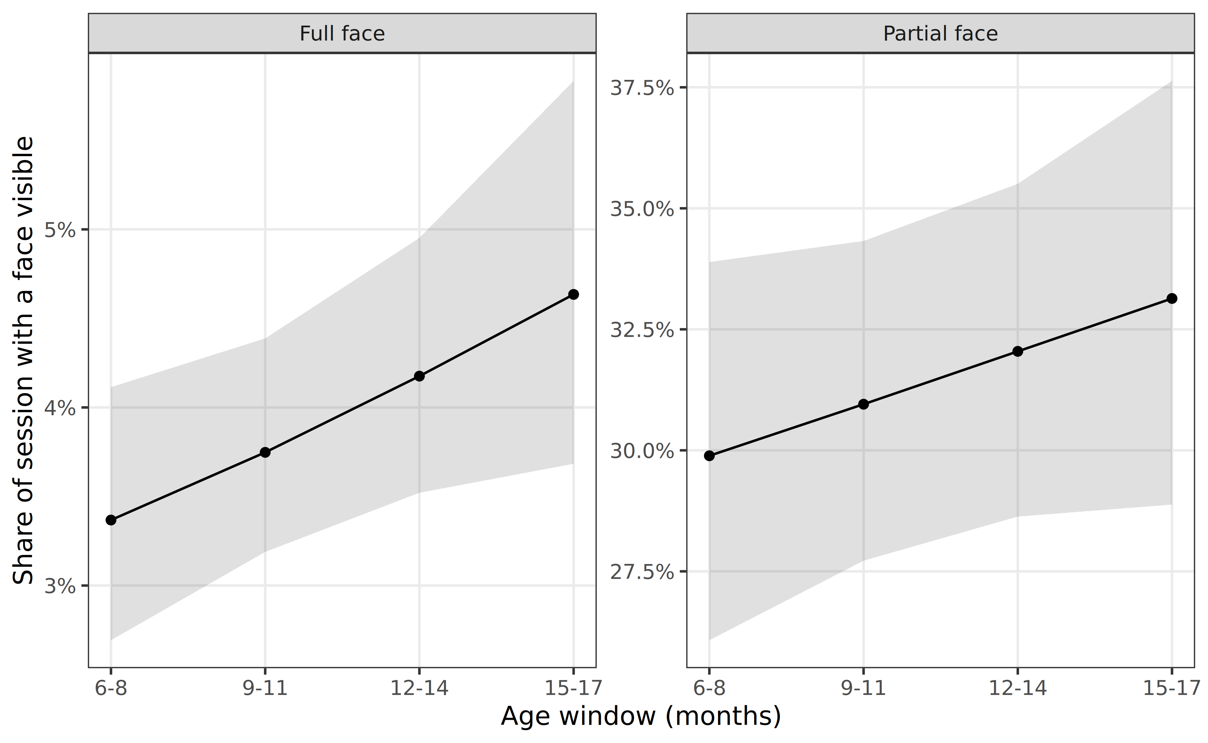

ggsave("fig_presence.png", fig_presence, width = 6.5, height = 4, dpi = 300)

IN-TEXT NUMBERS

vd_part <- variance_decomposition(part_null)
vd_full <- variance_decomposition(full_null)

list(
  n_sessions_part   = sum(!is.na(df_part$pct_part)),
  n_sessions_full   = sum(!is.na(df_full$pct_full)),
  n_infants         = n_distinct(df_part$subject),
  part_mean         = mean(df_part$pct_part, na.rm = TRUE),
  part_median       = median(df_part$pct_part, na.rm = TRUE),
  full_mean         = mean(df_full$pct_full, na.rm = TRUE),
  full_median       = median(df_full$pct_full, na.rm = TRUE),
  part_icc          = vd_part$ICC_decomposed,
  full_icc          = vd_full$ICC_decomposed
) |>
  enframe(name = "quantity", value = "value") |>
  mutate(value = map_chr(value, \(x) format(unlist(x), digits = 3))) |>
  print(n = Inf)

# A tibble: 9 × 2
  quantity        value 
  <chr>           <chr> 
1 n_sessions_part 135   
2 n_sessions_full 136   
3 n_infants       44    
4 part_mean       0.318 
5 part_median     0.307 
6 full_mean       0.04  
7 full_median     0.0304
8 part_icc        0.384 
9 full_icc        0.201 

cat(sprintf(
"## Key takeaways

1. **Faces are rare in infants' view.** A full face was visible for a median of
   %.1f%% of the session; a partial face for %.1f%%.
2. **Infants differ from one another.** The intercept-only models attribute
   %.0f%% (partial) and %.0f%% (full) of the variance to stable between-infant
   differences.
",
  100 * median(df_full$pct_full, na.rm = TRUE),
  100 * median(df_part$pct_part, na.rm = TRUE),
  100 * vd_part$ICC_decomposed,
  100 * vd_full$ICC_decomposed
))

Key takeaways

1. Faces are rare in infants’ view. A full face was visible for a median of 3.0% of the session; a partial face for 30.7%.
2. Infants differ from one another. The intercept-only models attribute 38% (partial) and 20% (full) of the variance to stable between-infant differences.

SUPPLEMENT

S1. Distributions

bind_rows(
  df_part |> transmute(pct = pct_part, Measure = "Partial face"),
  df_full |> transmute(pct = pct_full, Measure = "Full face")
) |>
  drop_na(pct) |>
  ggplot(aes(x = pct)) +
  geom_histogram(color = "white", breaks = seq(0, 1, 0.025)) +
  facet_wrap(~Measure, scales = "free_y") +
  scale_x_continuous(breaks = seq(0, 1, 0.2), labels = scales::percent) +
  labs(x = "Share of session with a face visible", y = "Sessions") +
  theme_bw(base_size = 10)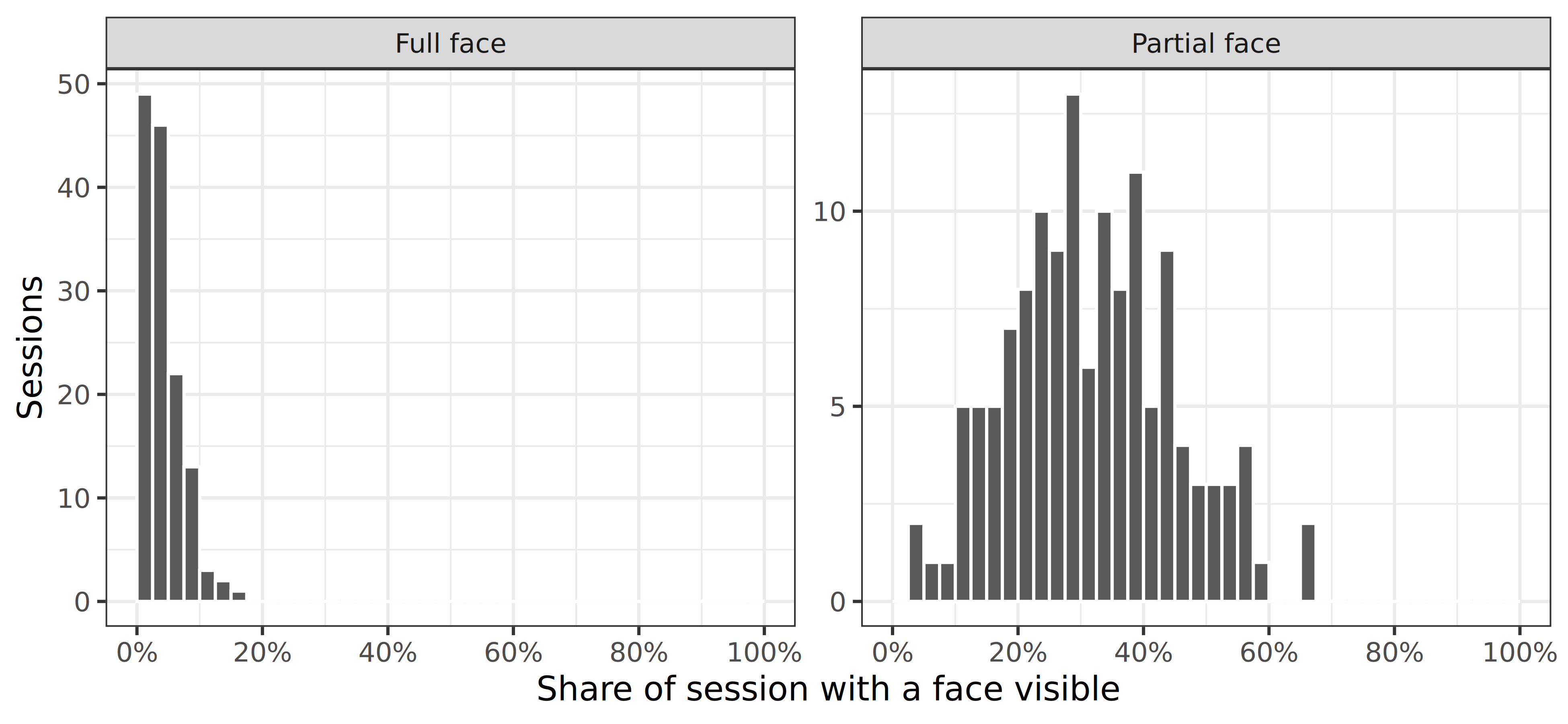

S2. Monotonic models

The linear models assume evenly spaced age effects. The monotonic models relax that, allowing the spacing between windows to be estimated.

model_parameters(part_monotonic, effects = "fixed") |> print_md()

Fixed Effects

Parameter	Median	95% CI	pd	Rhat	ESS (tail)
(Intercept)	-0.85	(-1.06, -0.65)	100%	1.001	2131
mowindow	0.04	(-0.03, 0.12)	86.70%	1.000	2776

model_parameters(full_monotonic, effects = "fixed") |> print_md()

Fixed Effects

Parameter	Median	95% CI	pd	Rhat	ESS (tail)
(Intercept)	-3.36	(-3.62, -3.13)	100%	1.000	2844
mowindow	0.10	(-7.11e-03, 0.21)	96.88%	1.000	2392

S3. Model checks

pp_check(part_linear, ndraws = 50)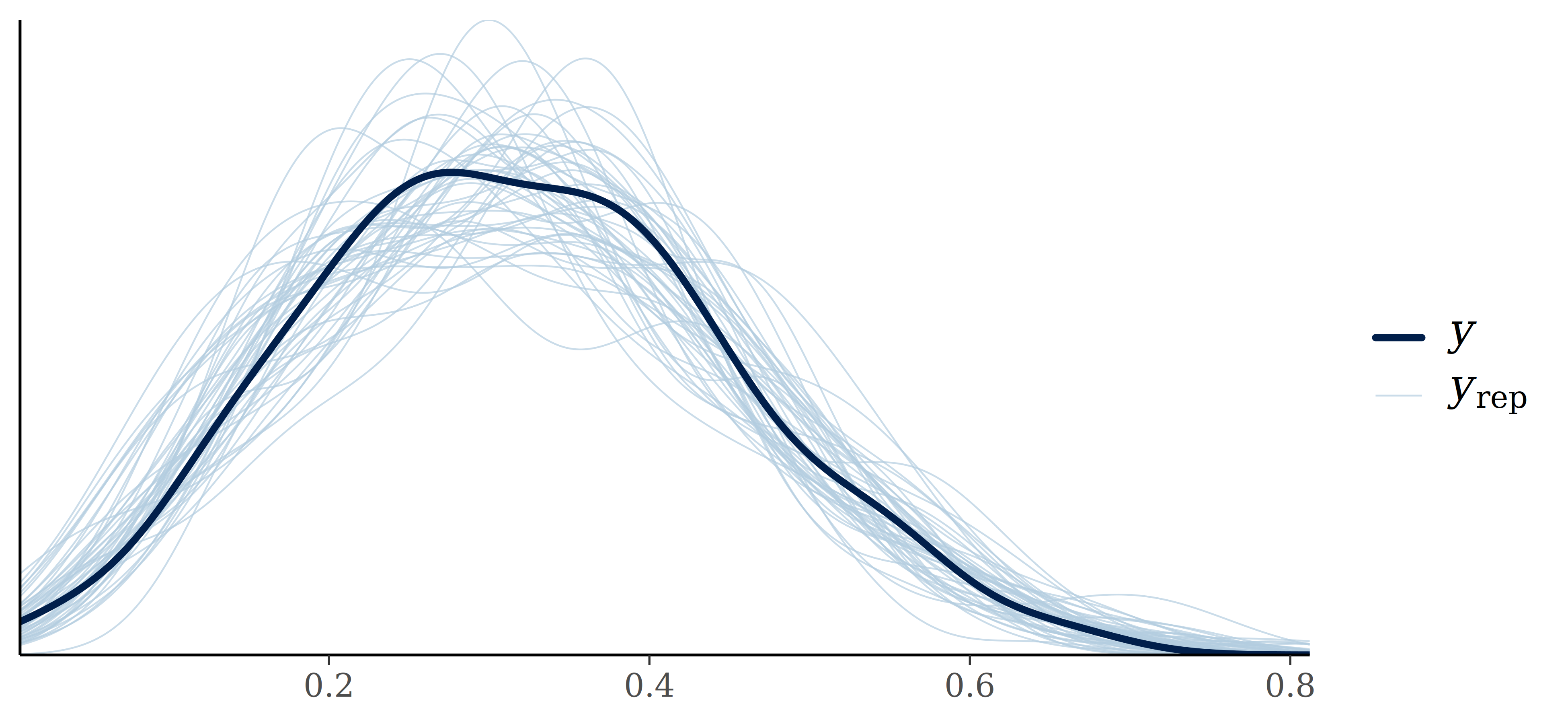

pp_check(full_linear, ndraws = 50)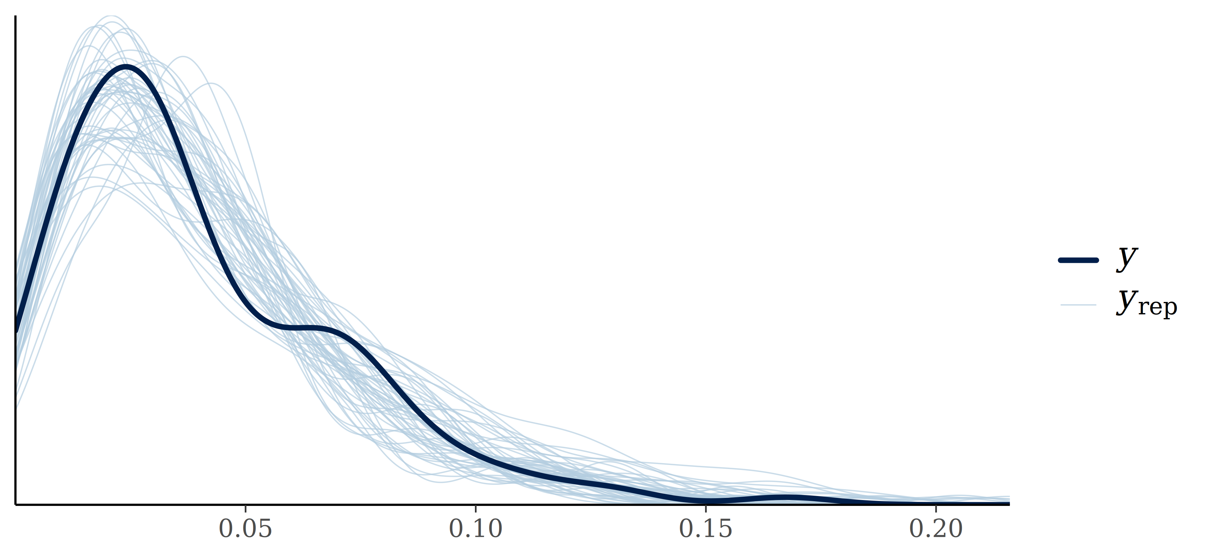

S4. Variance decomposition

vd_part

# Random Effect Variances and ICC

Conditioned on: all random effects

## Variance Ratio (comparable to ICC)
Ratio: 0.38  CI 95%: [0.11 0.57]

## Variances of Posterior Predicted Distribution
Conditioned on fixed effects: 0.01  CI 95%: [0.01 0.02]
Conditioned on rand. effects: 0.02  CI 95%: [0.01 0.02]

## Difference in Variances
Difference: 0.01  CI 95%: [0.00 0.01]

vd_full

# Random Effect Variances and ICC

Conditioned on: all random effects

## Variance Ratio (comparable to ICC)
Ratio: 0.20  CI 95%: [-0.34 0.52]

## Variances of Posterior Predicted Distribution
Conditioned on fixed effects: 0.00  CI 95%: [0.00 0.00]
Conditioned on rand. effects: 0.00  CI 95%: [0.00 0.00]

## Difference in Variances
Difference: 0.00  CI 95%: [-0.00 0.00]